5  Rcpp

When parallel computing is not enough, you can boost your R code using a lower-level programming language¹ like C++, C, or Fortran. With R itself written in C, it provides access points (APIs) to connect C++/C/Fortran functions to R. Although not impossible, using lower-level languages to enhance R can be cumbersome; Rcpp (Eddelbuettel and François 2011; Eddelbuettel 2013; Eddelbuettel and Balamuta 2018) can make things very easy. This chapter shows you how to use Rcpp–the most popular way to connect C++ with R–to accelerate your R code.

5.1 Before we start

1. You need to have Rcpp installed in your system:

   install.packages("Rcpp")

2. You need to have a compiler

   • Windows: You can download Rtools from here.

   • MacOS: It is a bit complicated… Here are some options:

     • CRAN’s manual to get the clang, clang++, and gfortran compilers here.

     • A great guide by the coatless professor here

And that’s it!

5.2 R is great, but…

• The problem:

  • As we saw, R is very fast… once vectorized

  • What to do if your model cannot be vectorized?

• The solution: Use C/C++/Fotran! It works with R!

• The problem to the solution: What R user knows any of those!?

• R has had an API (application programming interface) for integrating C/C++ code with R for a long time.

• Unfortunately, it is not very straightforward

5.3 Enter Rcpp

• One of the most important R packages on CRAN.

• As of January 22, 2023, about 50% of CRAN packages depend on it (directly or not).

• From the package description:

The ‘Rcpp’ package provides R functions as well as C++ classes which offer a seamless integration of R and C++

5.4 Why bother?

• To draw ten numbers from a normal distribution with sd = 100.0 using R C API:

  SEXP stats = PROTECT(R_FindNamespace(mkString("stats")));
  SEXP rnorm = PROTECT(findVarInFrame(stats, install("rnorm")));
  SEXP call = PROTECT(
    LCONS( rnorm, CONS(ScalarInteger(10), CONS(ScalarReal(100.0),
    R_NilValue))));
  SET_TAG(CDDR(call),install("sd"));
  SEXP res = PROTECT(eval(call, R_GlobalEnv));
  UNPROTECT(4);
  return res;

• Using Rcpp:

  Environment stats("package:stats");
  Function rnorm = stats["rnorm"];
  return rnorm(10, Named("sd", 100.0));

5.5 Example 1: Looping over a vector

#include<Rcpp.h>
using namespace Rcpp;
// [[Rcpp::export]]
NumericVector add1(NumericVector x) {
  NumericVector ans(x.size());
  for (int i = 0; i < x.size(); ++i)
    ans[i] = x[i] + 1;
  return ans;
}

add1(1:10)

 [1]  2  3  4  5  6  7  8  9 10 11

Make it sweeter by adding some “sugar” (the Rcpp kind)

#include<Rcpp.h>
using namespace Rcpp;
// [[Rcpp::export]]
NumericVector add1Cpp(NumericVector x) {
  return x + 1;
}

add1Cpp(1:10)

 [1]  2  3  4  5  6  7  8  9 10 11

5.6 How much fast?

Compared to this:

add1R <- function(x) {
  for (i in 1:length(x))
    x[i] <- x[i] + 1
  x
}
microbenchmark::microbenchmark(add1R(1:1000), add1Cpp(1:1000))

Unit: microseconds
            expr    min      lq     mean  median      uq      max neval cld
   add1R(1:1000) 34.909 36.4040 52.46721 36.8550 38.0415 1541.597   100  a 
 add1Cpp(1:1000)  2.246  2.6205 11.78040  3.2645  5.4385  770.870   100   b

5.7 Main differences between R and C++

1. One is compiled, and the other interpreted

2. Indexing objects: In C++ the indices range from 0 to (n - 1), whereas in R is from 1 to n.

3. All expressions end with a ; (optional in R).

4. In C++ object need to be declared, in R not (dynamic).

5.8 C++/Rcpp fundamentals: Types

Besides C-like data types (double, int, char, and bool), we can use the following types of objects with Rcpp:

• Matrices: NumericMatrix, IntegerMatrix, LogicalMatrix, CharacterMatrix

• Vectors: NumericVector, IntegerVector, LogicalVector, CharacterVector

• And more!: DataFrame, List, Function, Environment

5.9 Parts of “an Rcpp program”

#include<Rcpp.h>
using namespace Rcpp
// [[Rcpp::export]]
NumericVector add1(NumericVector x) {
  NumericVector ans(x.size());
  for (int i = 0; i < x.size(); ++i)
    ans[i] = x[i] + 1;
  return ans;
}

Line by line, we see the following:

1. The #include<Rcpp.h> is similar to library(...) in R, it brings in all that we need to write C++ code for Rcpp.

2. using namespace Rcpp is somewhat similar to detach(...). This simplifies syntax. If we don’t include this, all calls to Rcpp members need to be explicit, e.g., instead of typing NumericVector, we would need to type Rcpp::NumericVector

3. The // starts a comment in C++, in this case, the // [[Rcpp::export]] comment is a flag Rcpp uses to “export” this C++ function to R.

4. It is the first part of the function definition. We are creating a function that returns a NumericVector, is called add1, has a single input element named x that is also a NumericVector.

5. Here, we are declaring an object called ans, which is a NumericVector with an initial size equal to the size of x. Notice that .size() is called a “member function” of the x object, which is of class NumericVector.

6. We are declaring a for-loop (three parts):

   1. int i = 0 We declare the variable i, an integer, and initialize it at 0.

   2. i < x.size() This loop will end when i’s value is at or above the length of x.

   3. ++i At each iteration, i will increment in one unit.

7. ans[i] = x[i] + 1 set the i-th element of ans equal to the i-th element of x plus 1.

8. return ans exists the function returning the vector ans.

Now, where to execute/run this?

• You can use the sourceCpp function from the Rcpp package to run .cpp scripts (this is what I do most of the time).
• There’s also cppFunction, which allows compiling a single function.
• Write an R package that works with Rcpp.

For now, let’s use the first option.

5.10 Example running .cpp file

Imagine that we have the following file named norm.cpp

#include <Rcpp.h>
using namespace Rcpp;
// [[Rcpp::export]]
double normRcpp(NumericVector x) {
  
  return sqrt(sum(pow(x, 2.0)));
  
}

We can compile and obtain this function using this line Rcpp::sourceCpp("norm.cpp"). Once compiled, a function called normRcpp will be available in the current R session.

5.11 Your turn

5.11.1 Problem 1: Adding vectors

1. Using what you have just learned about Rcpp, write a function to add two vectors of the same length. Use the following template

#include <Rcpp.h>
using namespace Rcpp;
// [[Rcpp::export]]
NumericVector add_vectors([declare vector 1], [declare vector 2]) {
  
  ... magick ...
  
  return [something];
}

2. Now, we have to check for lengths. Use the stop function to make sure lengths match. Add the following lines in your code

if ([some condition])
  stop("an arbitrary error message :)");

5.11.2 Problem 2: Fibonacci series

Each element of the sequence is determined by the following:

\[ F(n) = \left\{\begin{array}{ll} n, & \mbox{ if }n \leq 1\\ F(n - 1) + F(n - 2), & \mbox{otherwise} \end{array}\right. \]

Using recursions, we can implement this algorithm in R as follows:

fibR <- function(n) {
  if (n <= 1)
    return(n)
  fibR(n - 1) + fibR(n - 2)
}
# Is it working?
c(
  fibR(0), fibR(1), fibR(2),
  fibR(3), fibR(4), fibR(5),
  fibR(6)
)

[1] 0 1 1 2 3 5 8

Now, let’s translate this code into Rcpp and see how much speed boost we get!

5.11.3 Problem 2: Fibonacci series (solution)

Code

#include <Rcpp.h>
// [[Rcpp::export]]
int fibCpp(int n) {
  if (n <= 1)
    return n;
  
  return fibCpp(n - 1) + fibCpp(n - 2);
  
}

microbenchmark::microbenchmark(fibR(20), fibCpp(20))

Unit: microseconds
       expr      min       lq       mean   median       uq      max neval cld
   fibR(20) 5350.894 5643.050 5982.69115 5724.878 5810.474 8855.542   100  a 
 fibCpp(20)   11.928   12.479   24.21755   15.318   21.728  706.360   100   b

5.12 RcppArmadillo and OpenMP

• Friendlier than RcppParallel… at least for ‘I-use-Rcpp-but-don’t-actually-know-much-about-C++’ users (like myself!).

• Must run only ‘Thread-safe’ calls, so calling R within parallel blocks can cause problems (almost all the time).

• Use arma objects, e.g. arma::mat, arma::vec, etc. Or, if you are used to them std::vector objects as these are thread-safe.

• Pseudo Random Number Generation is not very straightforward… But C++11 has a nice set of functions that can be used together with OpenMP

• Need to think about how processors work, cache memory, etc. Otherwise, you could get into trouble… if your code is slower when run in parallel, then you probably are facing false sharing

• If R crashes… try running R with a debugger (see Section 4.3 in Writing R extensions):

  ~$ R --debugger=valgrind

5.12.1 RcppArmadillo and OpenMP workflow

1. Tell Rcpp that you need to include that in the compiler:

   #include <omp.h>
   // [[Rcpp::plugins(openmp)]]

2. Within your function, set the number of cores, e.g

   // Setting the cores
   omp_set_num_threads(cores);

3. Tell the compiler that you’ll be running a block in parallel with OpenMP

   #pragma omp [directives] [options]
   {
     ...your neat parallel code...
   }

   You’ll need to specify how OMP should handle the data:

   • shared: Default, all threads access the same copy.
   • private: Each thread has its own copy, uninitialized.
   • firstprivate Each thread has its own copy, initialized.
   • lastprivate Each thread has its own copy. The last value used is returned.

   Setting default(none) is a good practice.

4. Compile!

5.12.2 Ex 5: RcppArmadillo + OpenMP

Our own version of the dist function… but in parallel!

#include <omp.h>
#include <RcppArmadillo.h>
// [[Rcpp::depends(RcppArmadillo)]]
// [[Rcpp::plugins(openmp)]]
using namespace Rcpp;
// [[Rcpp::export]]
arma::mat dist_par(const arma::mat & X, int cores = 1) {
  
  // Some constants
  int N = (int) X.n_rows;
  int K = (int) X.n_cols;
  
  // Output
  arma::mat D(N,N);
  D.zeros(); // Filling with zeros
  
  // Setting the cores
  omp_set_num_threads(cores);
  
#pragma omp parallel for shared(D, N, K, X) default(none)
  for (int i=0; i<N; ++i)
    for (int j=0; j<i; ++j) {
      for (int k=0; k<K; k++) 
        D.at(i,j) += pow(X.at(i,k) - X.at(j,k), 2.0);
      
      // Computing square root
      D.at(i,j) = sqrt(D.at(i,j));
      D.at(j,i) = D.at(i,j);
    }
      
  
  // My nice distance matrix
  return D;
}

# Simulating data
set.seed(1231)
K <- 5000
n <- 500
x <- matrix(rnorm(n*K), ncol=K)
# Are we getting the same?
table(as.matrix(dist(x)) - dist_par(x, 4)) # Only zeros

     0 
250000 

# Benchmarking!
microbenchmark::microbenchmark(
  dist(x),                # stats::dist
  dist_par(x, cores = 1), # 1 core
  dist_par(x, cores = 2), # 2 cores
  dist_par(x, cores = 4), # 4 cores
  times = 1, 
  unit = "ms"
)

Unit: milliseconds
                   expr      min       lq     mean   median       uq      max
                dist(x) 2188.525 2188.525 2188.525 2188.525 2188.525 2188.525
 dist_par(x, cores = 1) 2424.293 2424.293 2424.293 2424.293 2424.293 2424.293
 dist_par(x, cores = 2) 1863.913 1863.913 1863.913 1863.913 1863.913 1863.913
 dist_par(x, cores = 4) 1209.131 1209.131 1209.131 1209.131 1209.131 1209.131
 neval
     1
     1
     1
     1

5.12.3 Ex 6: The future

• future is an R package that was designed “to provide a very simple and uniform way of evaluating R expressions asynchronously using various resources available to the user.”

• future class objects are either resolved or unresolved.

• If queried, Resolved values are return immediately, and Unresolved values will block the process (i.e. wait) until it is resolved.

• Futures can be parallel/serial, in a single (local or remote) computer, or a cluster of them.

Let’s see a brief example

library(future)
plan(multicore)
# We are creating a global variable
a <- 2
# Creating the futures has only the overhead (setup) time
system.time({
  x1 %<-% {Sys.sleep(3);a^2}
  x2 %<-% {Sys.sleep(3);a^3}
})
##    user  system elapsed 
##   0.018   0.012   0.030
# Let's just wait 5 seconds to make sure all the cores have returned
Sys.sleep(3)
system.time({
  print(x1)
  print(x2)
})
## [1] 4
## [1] 8
##    user  system elapsed 
##   0.003   0.000   0.003

5.12.4 Bonus track 1: Simulating \(\pi\)

• We know that \(\pi = \frac{A}{r^2}\). We approximate it by randomly adding points \(x\) to a square of size 2 centered at the origin.

• So, we approximate \(\pi\) as \(\Pr\{\|x\| \leq 1\}\times 2^2\)

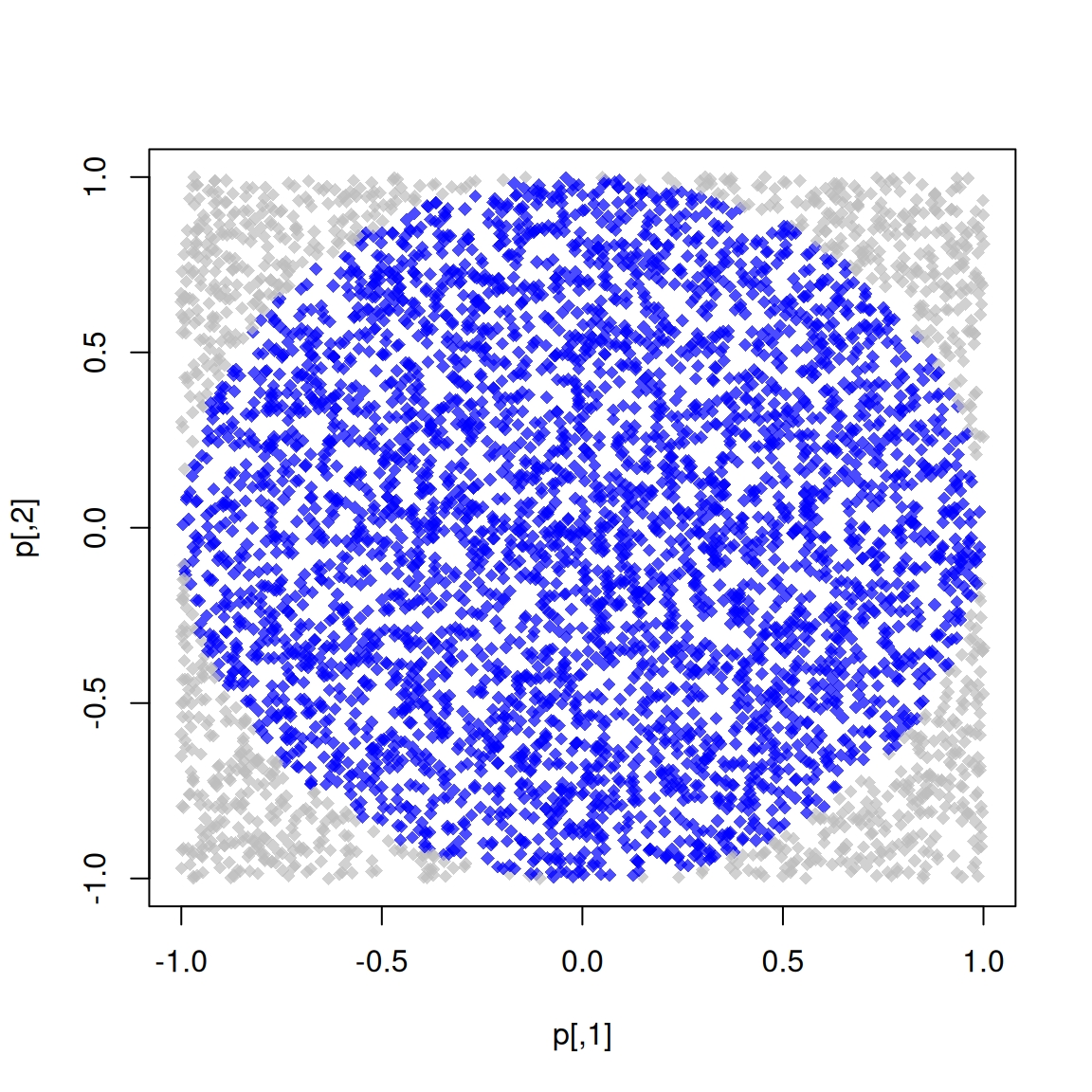
The R code to do this

pisim <- function(i, nsim) {  # Notice we don't use the -i-
  # Random points
  ans  <- matrix(runif(nsim*2), ncol=2)
  
  # Distance to the origin
  ans  <- sqrt(rowSums(ans^2))
  
  # Estimated pi
  (sum(ans <= 1)*4)/nsim
}

library(parallel)
# Setup
cl <- makePSOCKcluster(4L)
clusterSetRNGStream(cl, 123)
# Number of simulations we want each time to run
nsim <- 1e5
# We need to make -nsim- and -pisim- available to the
# cluster
clusterExport(cl, c("nsim", "pisim"))
# Benchmarking: parSapply and sapply will run this simulation
# a hundred times each, so at the end we have 1e5*100 points
# to approximate pi
microbenchmark::microbenchmark(
  parallel = parSapply(cl, 1:100, pisim, nsim=nsim),
  serial   = sapply(1:100, pisim, nsim=nsim),
  times    = 1
)

Unit: milliseconds
     expr      min       lq     mean   median       uq      max neval
 parallel 295.0158 295.0158 295.0158 295.0158 295.0158 295.0158     1
   serial 405.3509 405.3509 405.3509 405.3509 405.3509 405.3509     1

---

ans_par <- parSapply(cl, 1:100, pisim, nsim=nsim)
ans_ser <- sapply(1:100, pisim, nsim=nsim)
stopCluster(cl)

     par      ser        R 
3.141762 3.141266 3.141593 

5.13 See also

• Package parallel
• Using the iterators package
• Using the foreach package
• 32 OpenMP traps for C++ developers
• The OpenMP API specification for parallel programming
• ‘openmp’ tag in Rcpp gallery
• OpenMP tutorials and articles

For more, check out the CRAN Task View on HPC

Eddelbuettel, Dirk. 2013. Seamless R and C++ Integration with Rcpp. New York: Springer. https://doi.org/10.1007/978-1-4614-6868-4.

Eddelbuettel, Dirk, and James Joseph Balamuta. 2018. “Extending extitR with extitC++: A Brief Introduction to extitRcpp.” The American Statistician 72 (1): 28–36. https://doi.org/10.1080/00031305.2017.1375990.

Eddelbuettel, Dirk, and Romain François. 2011. “Rcpp: Seamless R and C++ Integration.” Journal of Statistical Software 40 (8): 1–18. https://doi.org/10.18637/jss.v040.i08.

---

1. In general, a low-level programming language is “a programming language that provides little or no abstraction from a computer’s set architecture […]” (wiki), yet, here we use that term to refer to programming languages that are closer to machine code than what R is.